How to do a VLOOKUP to the left of the search column? Two solutions are possible, but not with VLOOKUP.

1. VLOOKUP Limitation
   The VLOOKUP function can only retrieve a value to the right of the lookup column. There is no parameter to read to the left.
2. Modern solution: XLOOKUP
   To overcome this limitation, Microsoft created the XLOOKUP function. It allows you to search in any column, left or right. Its use is more flexible and its syntax simpler.
3. Classic alternative: INDEX + EQUIV
   Before XLOOKUP, the only way to read left was to combine INDEX and MATCH. This combination remains effective but can seem complex to master for beginners.

VLOOKUP only reads to the right ⛔

The VLOOKUP function allows you to search for data in an array by returning data always located to the right of the search column. But there are 2 other search functions that allow you to get around this problem.

We will see how to retrieve the country name (column A) using the country code (column B)

Solution with SEARCHEX

La LOOKUP function is one of the newest functions developed by Microsoft in Excel 365. It improves the shortcomings observed with the VLOOKUP function, like search on the left.

1. Start by writing the name of the XLOOKUP function
2. Then indicate the cell containing the element to search for
3. Select only the column where is the item to search for (here, column B)
4. Finally, select the column to return (here, column A)

The formula in this example is:

=RECHERCHEX(H2;B2:B233;A2:A233)

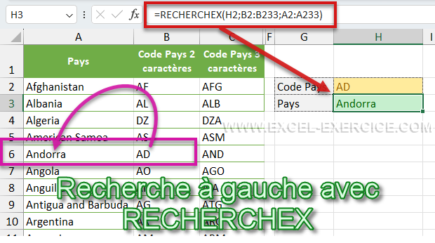
• With XLOOKUP, there are only 2 columns to select, the search column and the column to return

Solution with INDEX and EQUIV

If you don't work with Excel 365 or Excel Online, here's how to search left.

1. We will start by writing the INDEX function.
2. As a first parameter, we will select only the country names column, the information we are looking for =INDEX($A$2:$A$233
3. Then, for the second argument, we will utiliser the MATCH function. This function returns the position of an element in a list.
4. As we seek the AD code position and our list, we will write =EQUIV($H$2;$B$2:$B$233;0)
5. The 0 at the end indicates that we are doing an exact search.
6. Finally, we add this EQUIV formula as the second argument of the INDEX function

=INDEX($A$2:$A$233;EQUIV($H$2;$B$2:$B$233;0))

Related Articles

• Understanding the VLOOKUP function with a quiz
• Why does the VLOOKUP function return #N/A?
• XLOOKUP, the replacement for the VLOOKUP function
• MATCH function in Excel
• INDEX function in Excel
• Exercise on the INDEX and EQUIV functions

Explanatory video

The following video shows you the technique and you have the explanations afterwards